Programming examples
Example 1
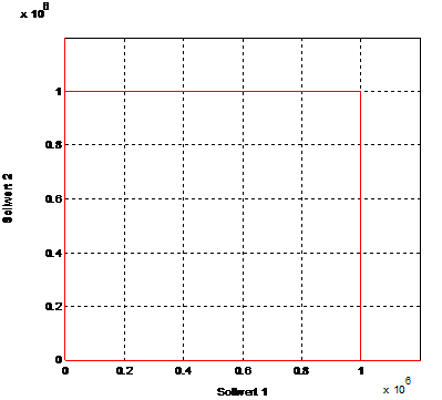
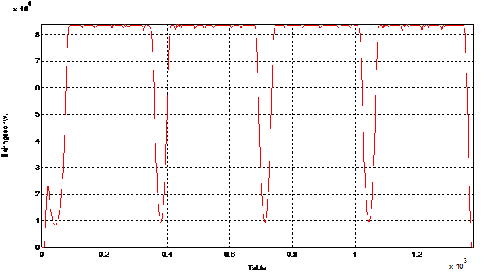
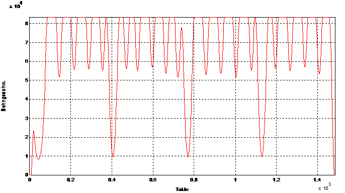
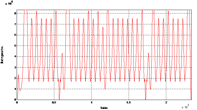
In the test program below, a square with an edge length of 100 mm is moved. Each side is segmented into 100 single blocks. Based on a time ahead of 2 seconds, as values become increasingly smaller it becomes apparent that the contouring speed can no longer be kept constant due to the pulsating supply of blocks.
% Quadrat.nc
#SLOPE [TYPE=HSC]
G133 100
V.G.MAX_TIME_AHEAD = 2 ;seconds
G00 G90 X0 Y0
P40 = 5000
P30=100.0 (* Side length of square *)
P20 = 100 (* Number of blocks on side length*)
P10 = P30/P20
$FOR P1=1,P20, 1
N[P1]G01 G91 XP10 FP40
$ENDFOR
G90
$FOR P1=1,P20, 1
N[P1+1000]G01 G91 YP10
$ENDFOR
G90
$FOR P1=1,P20, 1
N[P1+2000]G01 G91 X-P10
$ENDFOR
G90
$FOR P1=1,P20, 1
N[P1+3000]G01 G91 Y-P10
$ENDFOR
G90
V.G.MAX_TIME_AHEAD = 0 ;seconds
M30

Example 2
In default mode the mean feed velocity is always included in the calculation of time ahead. This function can be deactivated by the channel parameter P-CHAN-00428 (calc_average_feed_ahead) to run in programs and for diagnostic purposes.
The idealised test program listed below examines and illustrates the influence of the mean feed velocity on the accuracy of the actual time ahead.
Test 1:
Program with 40 mm linear blocks and feed limits, time ahead 2s
%average_feed_ahead_1
F60000 G01
V.G.MAX_TIME_AHEAD = 2
#VECTOR LIMIT ON [VEL=20000]
$FOR P1=0,100,1
G91 X40
$ENDFOR
G91 Y10
#VECTOR LIMIT ON [VEL=40000]
$FOR P1=0,100,1
G91 X-40
$ENDFOR
G91 Y-10
M30
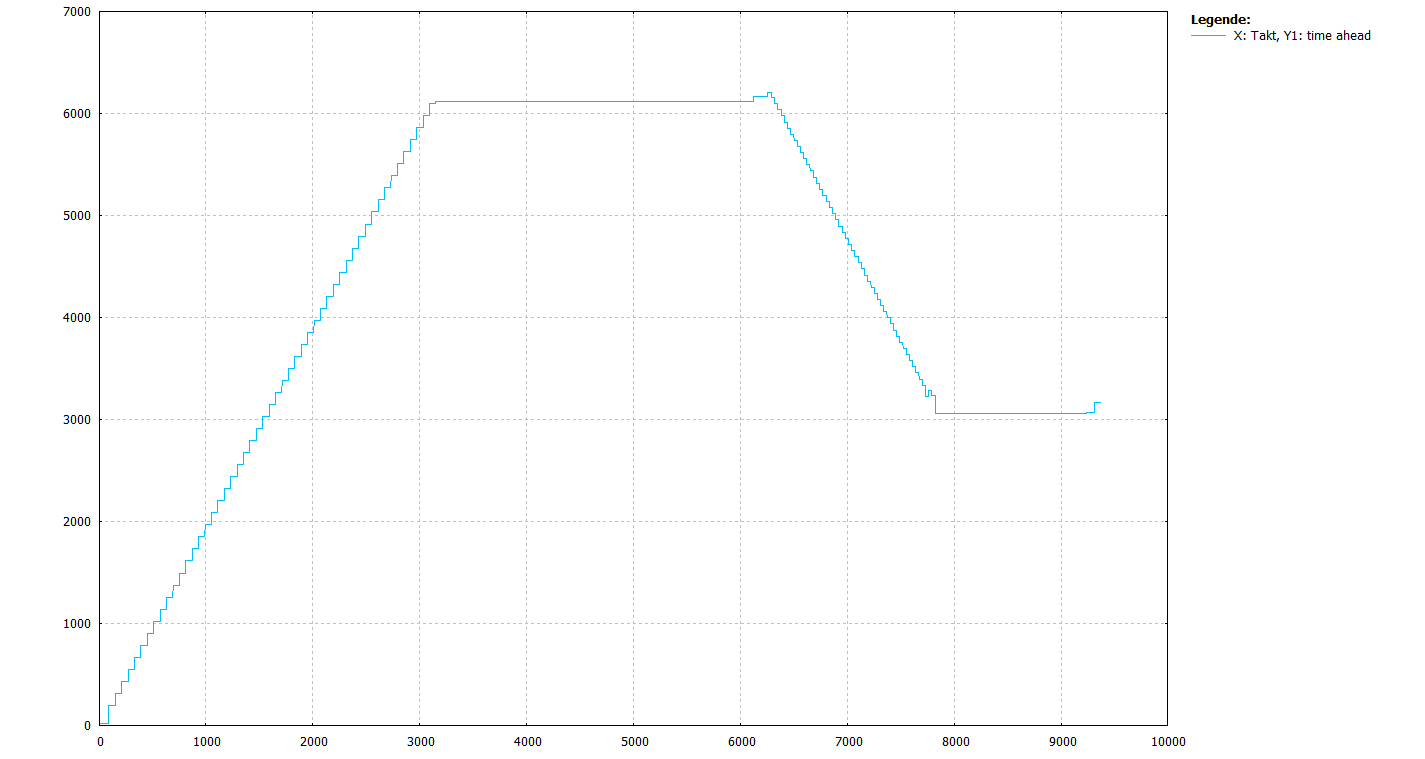
Block supply is ensured by the long geometry blocks (40mm). The velocity influence by #VECTOR LIMIT is not considered in the time ahead calculation due to P-CHAN-00428 = 0. The required time ahead of 2 s is exceeded by a considerable amount
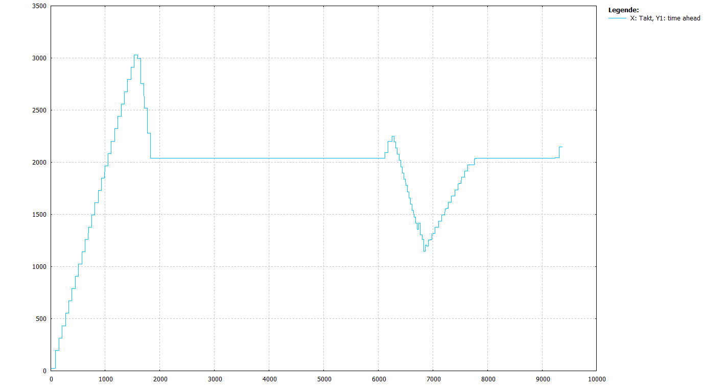
At start a slight excess occurs but this is re-adjusted. The required time ahead of 2 s is basically maintained
Test 2:
Program with 10 mm (short) linear blocks and feed limits, time ahead 2s
%average_feed_ahead_2
F60000 G01
V.G.MAX_TIME_AHEAD = 2
#VECTOR LIMIT ON [VEL=20000]
$FOR P1=0,400,1
G91 X10
$ENDFOR
G91 Y10
#VECTOR LIMIT ON [VEL=40000]
$FOR P1=0,400,1
G91 X-10
$ENDFOR
G91 Y-10
M30
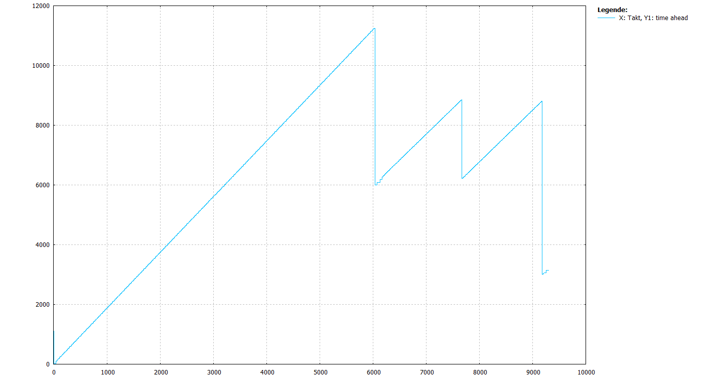
Due to the short geometry blocks (10mm) the priority for interpolation is to ensure block supply. Stable block ahead limiting is not achieved. The required time ahead of 2 s is exceeded by a considerable amount.
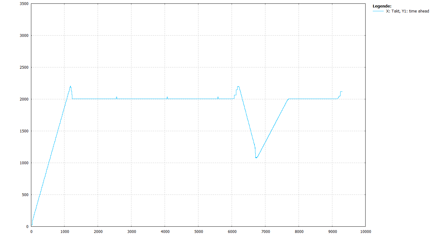
At start a slight excess occurs but this is re-adjusted. The required lime ahead of 2 s is basically maintained.
Test 3:
Program with 40mm linear blocks without feed limits, time ahead 2s
%average_feed_ahead_3
F60000 G01
V.G.MAX_TIME_AHEAD = 2
$FOR P1=0,100,1
G91 X40
$ENDFOR
G91 Y10
$FOR P1=0,100,1
G91 X-40
$ENDFOR
G91 Y-10
M30
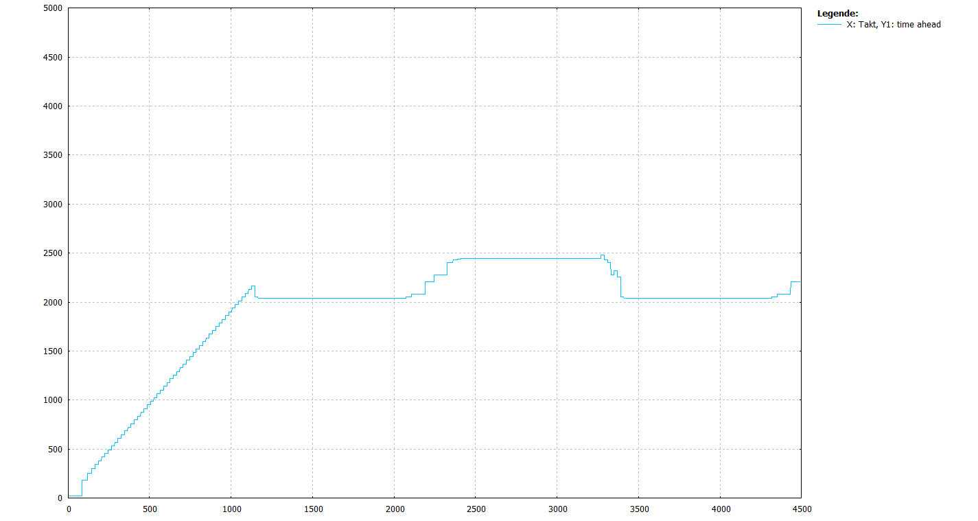
At start a slight excess occurs but this is re-adjusted. The required time ahead of 2 s is basically maintained.
Test 4:
Program with 10mm (short) linear blocks without feed limits, time ahead 2s
%average_feed_ahead_4
F60000 G01
V.G.MAX_TIME_AHEAD = 2
$FOR P1=0,400,1
G91 X10
$ENDFOR
G91 Y10
$FOR P1=0,400,1
G91 X-10
$ENDFOR
G91 Y-10
M30
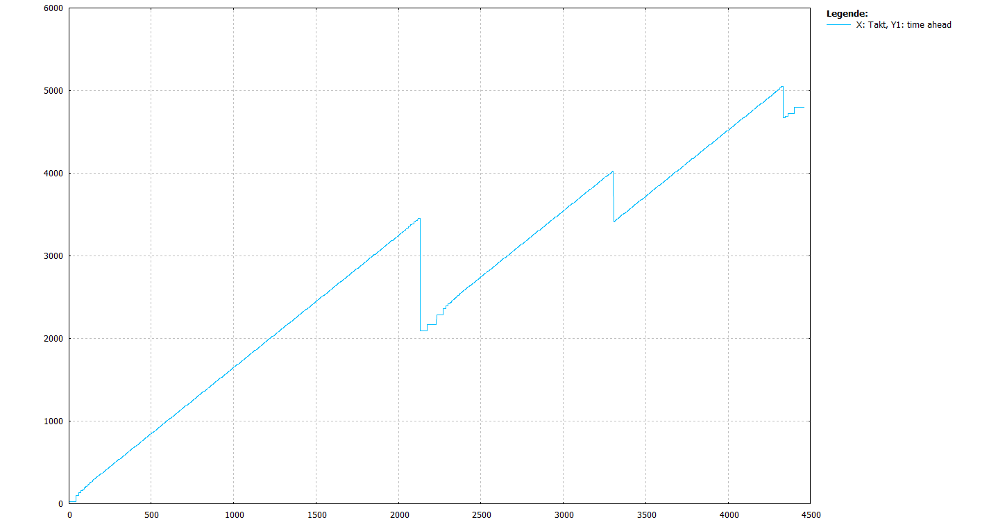
Due to the short geometry blocks (10mm) the priority for interpolation is to ensure block supply. Stable block ahead limiting is not achieved. The required time ahead of 2 s is exceeded by a considerable amount.
Example 3
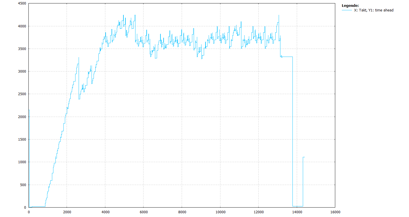
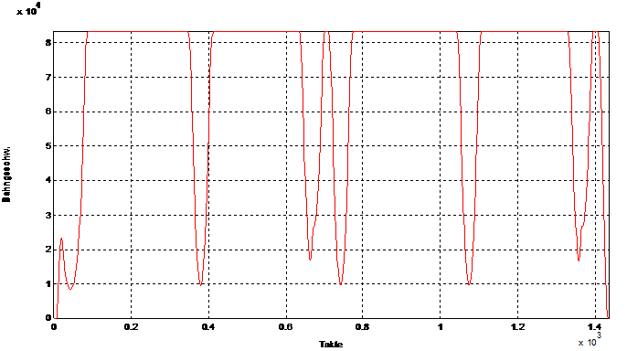
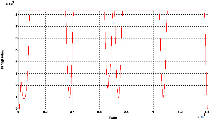
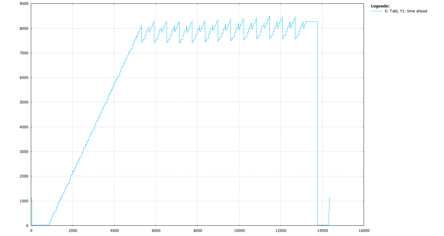
The graphics below show the curve of time ahead in an actual program. It features strongly fluctuating feeds (rapid traverse and normal feed). The resulting deceleration and acceleration phases cannot be exactly considered in advance when estimating block ahead limiting. This then results in a more or less strong deviation in the programmed time ahead.
Test 1:
Test 2:
